Introduction
M. Oren and S.K. Nayar proposed a diffuse BRDF in
Generalization of Lambert's Reflectance Model, Michael Oren, Shree K. Nayar, July 1994, Siggraph, pp. 239-246 that takes the roughness of a surface into account. This BRDF is often cited as too slow for realtime use, because of the sin and tan instructions in the equation. In this post I present a rewritten version of the equation which I'd like to call "
van Ouwerkerk's rewrite". The rewritten equation evaluates significantly faster on modern GPU's, making it more feasible to use the Oren Nayar BRDF in realtime applications.
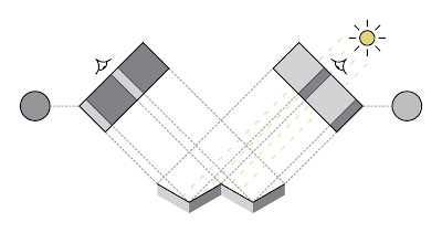 |
| Figure 1 - backscattering towards light source in V-cavities |
The Oren Nayar BRDF is based on mathematical analysis of light interacting with a surface consisting of V-cavities. In their work they predict that roughness results in more light being reflected back in the direction of the light source, which is illustrated in figure 1. This backscatter effect is contained in the resulting simplified Oren Nayar BRDF listed in equation 1.
 |
| Equation 1 - (simplified) Oren Nayar BRDF |
Angle range
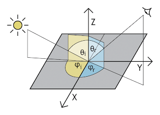 |
| Figure 2 - graphical overview of angles |
The incoming light direction is described by the angles θ
i and φ
i, while the reflected light direction is described by the angles θ
r and φ
r as illustrated in figure 2. The azimuth angles are described by φ
i and φ
r in a full circle from 0 to 2π on the plane of the surface. The zenith angles described by θ
i and θ
r are therefore always positive and range from 0 to π. Since light can't illuminate a surface from the back and we can't see a surface from the back, θ
i and θ
r are constrained to a meaningful range of 0 to π/2 as made explicit in equation 2.
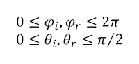 |
| Equation 2 - angles constrained to meaningful range |
Trigonometric identities
Our goal is to remove the sin and tan instructions from the Oren Nayar BRDF. Since a cos can often be replaced by a much faster dot product, we start by transforming the sin and tan instructions into cos instructions using the two trigonometric identities listed in equation 3. Note that the square root would mathematically have both a positive and a negative result. Since the zenith angles are constrained to the 0 to π/2 range, we can assume the positive result.
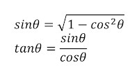 |
| Equation 3 - trigonometric identities |
This will transform the BRDF into the expanded form listed in equation 4. For easier reading, the part with the original sin and tan instructions is split into a separate part C of the equation.
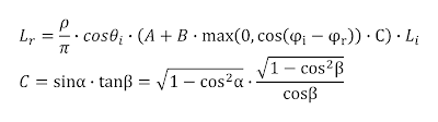 |
| Equation 4 - application of trigonometric identities |
Alpha and beta
 |
| Figure 3 - cosine from 0 to π/2 |
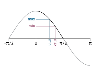
The dot product of two normalized vectors equals the cosine of the angle between them. This identity is very often used in computer graphics. The problem that arises with the Oren Nayar BRDF is that the angles α and β can't be readily expressed as an angle between two vectors. This prevents the use of a dot product instead of the more expensive cos instruction. In order to overcome this, we'll have to remove the min and max instructions inside the cos. If we look at the cosine function we see that it is strictly decreasing in the 0 to π/2 range as illustrated in figure 3. We can use this to move the min and max instructions outwards as listed in equation 5.
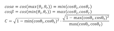 |
| Equation 5 - moving min and max outwards |
Minimum and maximum
Since both the minimum and the maximum of the incoming and reflected zenith angles are processed in the same way, we can apply another simplification as listed in equation 6. If one of the angles is the minimum, the other one is automatically the maximum. This means we can replace the mirrored min and max instructions with the two parameters contained in them. We can also combine the two square roots into one.
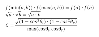 |
| Equation 6 - mirrored min and max |
Vector math
At this point we can replace all cosine functions with dot products and transform the equation into the vector math commonly found in realtime shaders. The final result is listed in equation 7.
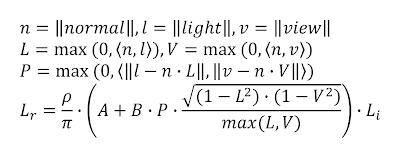 |
| Equation 7 - van Ouwerkerk's rewrite |
Implementation
The proposed equation is implemented in an HLSL pixel shader as shown in the listing below. The determination of the surface albedo and the amount of incoming light is not included in this listing as it depends on many other factors.
// Input vectors
float3 normal = normalize(input.normal);
float3 light = normalize(input.light);
float3 view = normalize(input.view);
// Roughness, A and B
float roughness = input.roughness;
float roughness2 = roughness * roughness;
float2 oren_nayar_fraction = roughness2 / (roughness2 + float2(0.33, 0.09));
float2 oren_nayar = float2(1, 0) + float2(-0.5, 0.45) * oren_nayar_fraction;
// Theta and phi
float2 cos_theta = saturate(float2(dot(normal, light), dot(normal, view)));
float2 cos_theta2 = cos_theta * cos_theta;
float sin_theta = sqrt((1-cos_theta2.x) * (1-cos_theta2.y));
float3 light_plane = normalize(light - cos_theta.x * normal);
float3 view_plane = normalize(view - cos_theta.y * normal);
float cos_phi = saturate(dot(light_plane, view_plane));
// Composition
float diffuse_oren_nayar = cos_phi * sin_theta / max(cos_theta.x, cos_theta.y);
float diffuse = cos_theta.x * (oren_nayar.x + oren_nayar.y * diffuse_oren_nayar);
Final words
I've hereby presented a faster way to evaluate the Oren Nayar BRDF specifically targeted at usage in realtime shaders. This document has been submitted as proposal to the GPU Pro 3 book.


in 'Equation 7' missing L ( cos_theta.x ) factor.
BeantwoordenVerwijderenEquation 7: L_r = cos( theta_i) rho/pi( ... ) L_i.
Se also implementation: float diffuse = cos_theta.x * ...